In R: Package microbenchmark (Example Code)
In this article, I’ll demonstrate how to use the microbenchmark package in R programming.
Setting up the Example
We load the packages: microbenchmark, ggplot2, data.table, and dplyr.
install.packages("microbenchmark") # Install & load microbenchmark package library("microbenchmark") install.packages("ggplot2") # Install & load ggplot2 package library("ggplot2") install.packages("data.table") # Install & load data.table library("data.table") install.packages("dplyr") # Install & load dplyr package library("dplyr") |
install.packages("microbenchmark") # Install & load microbenchmark package library("microbenchmark") install.packages("ggplot2") # Install & load ggplot2 package library("ggplot2") install.packages("data.table") # Install & load data.table library("data.table") install.packages("dplyr") # Install & load dplyr package library("dplyr")
For illustration, we use the iris dataset.
data(iris) # Load iris data set head(iris) # Print head of data # Sepal.Length Sepal.Width Petal.Length Petal.Width Species # 1 5.1 3.5 1.4 0.2 setosa # 2 4.9 3.0 1.4 0.2 setosa # 3 4.7 3.2 1.3 0.2 setosa # 4 4.6 3.1 1.5 0.2 setosa # 5 5.0 3.6 1.4 0.2 setosa # 6 5.4 3.9 1.7 0.4 setosa |
data(iris) # Load iris data set head(iris) # Print head of data # Sepal.Length Sepal.Width Petal.Length Petal.Width Species # 1 5.1 3.5 1.4 0.2 setosa # 2 4.9 3.0 1.4 0.2 setosa # 3 4.7 3.2 1.3 0.2 setosa # 4 4.6 3.1 1.5 0.2 setosa # 5 5.0 3.6 1.4 0.2 setosa # 6 5.4 3.9 1.7 0.4 setosa
We transform the dataset into a data.table object.
iris_dt <- as.data.table(iris) # Generate new data.table object |
iris_dt <- as.data.table(iris) # Generate new data.table object
Example: Calculating Group Medians
Now, we try different ways of calculating group medians. With the microbenchmark package, we can compare the performance of the different approaches. The microbenchmark package executes the different command for a predefined number of times. In the example below, we have 200 repetitions of each approach to have a more stable picture than just using few iterations.
bench_res <- microbenchmark("E1" = iris_dt %>% # Benchmarking the performance of different ways of calculating group medians group_by(Species) %>% filter(Sepal.Length <= 5) %>% summarize(median(Petal.Width)), "E2" = sapply(unique(iris_dt$Species), function (x){ median(iris_dt[iris_dt$Sepal.Length <= 5 & iris_dt$Species == x, Petal.Width]) }), "E3" = iris_dt[Sepal.Length <= 5, median(Petal.Width), Species], times = 200) bench_res # See results # Unit: milliseconds # expr min lq mean median uq max neval # E1 12.120701 14.02365 17.164829 15.797850 18.789552 36.391402 200 # E2 1.600201 1.86085 2.733440 2.183451 3.181651 12.679801 200 # E3 1.023701 1.16070 1.685625 1.268501 1.792151 7.435401 200 |
bench_res <- microbenchmark("E1" = iris_dt %>% # Benchmarking the performance of different ways of calculating group medians group_by(Species) %>% filter(Sepal.Length <= 5) %>% summarize(median(Petal.Width)), "E2" = sapply(unique(iris_dt$Species), function (x){ median(iris_dt[iris_dt$Sepal.Length <= 5 & iris_dt$Species == x, Petal.Width]) }), "E3" = iris_dt[Sepal.Length <= 5, median(Petal.Width), Species], times = 200) bench_res # See results # Unit: milliseconds # expr min lq mean median uq max neval # E1 12.120701 14.02365 17.164829 15.797850 18.789552 36.391402 200 # E2 1.600201 1.86085 2.733440 2.183451 3.181651 12.679801 200 # E3 1.023701 1.16070 1.685625 1.268501 1.792151 7.435401 200
You can see that the third approach, that is using data.table commands, is the most efficient way of calculating group means. It is much faster than the piping approach (E1).
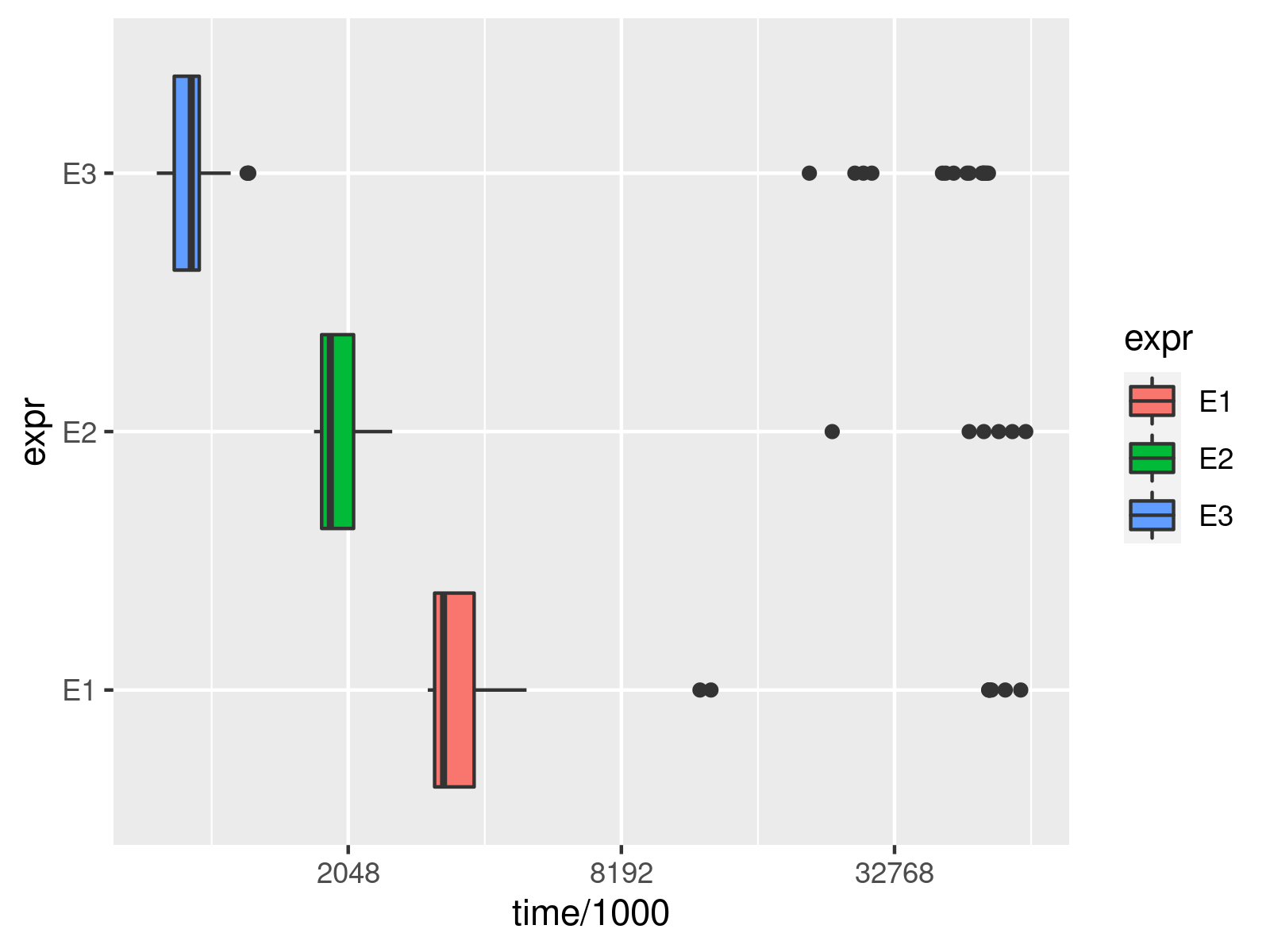
We can visualize the performance using ggplot2.
ggplot(bench_res, # Plot performance comparison aes(x = time/1000, y = expr, fill = expr)) + geom_boxplot() + scale_x_continuous(trans = 'log2') # ggplot2::autoplot(bench_res) |
ggplot(bench_res, # Plot performance comparison aes(x = time/1000, y = expr, fill = expr)) + geom_boxplot() + scale_x_continuous(trans = 'log2') # ggplot2::autoplot(bench_res)

The visualization makes the distribution of the computation time of the different approaches over the 200 evaluations even more clear and can also reveal heavy outliers.
Note: This article was created in collaboration with Anna-Lena Wölwer. Anna-Lena is a researcher and programmer who creates tutorials on statistical methodology as well as on the R programming language. You may find more info about Anna-Lena and her other articles on her profile page.

