In R: Generalized CV (GCV) | Example Code
This tutorial shows how to choose the penalty parameter of a spline using the generalized cross-validation (GCV) score in R programming.
Setting up the Example
We use packages SpatialExtremes and ggplot2.
install.packages("SpatialExtremes") # Install SpatialExtremes packages library("SpatialExtremes") # Load SpatialExtremes package install.packages("ggplot2") # Install ggplot2 packages library("ggplot2") # Load ggplot2 |
install.packages("SpatialExtremes") # Install SpatialExtremes packages library("SpatialExtremes") # Load SpatialExtremes package install.packages("ggplot2") # Install ggplot2 packages library("ggplot2") # Load ggplot2
We use the iris dataset for illustration.
data(iris) # Load iris data set head(iris) # Print head of data # Sepal.Length Sepal.Width Petal.Length Petal.Width Species # 1 5.1 3.5 1.4 0.2 setosa # 2 4.9 3.0 1.4 0.2 setosa # 3 4.7 3.2 1.3 0.2 setosa # 4 4.6 3.1 1.5 0.2 setosa # 5 5.0 3.6 1.4 0.2 setosa # 6 5.4 3.9 1.7 0.4 setosa |
data(iris) # Load iris data set head(iris) # Print head of data # Sepal.Length Sepal.Width Petal.Length Petal.Width Species # 1 5.1 3.5 1.4 0.2 setosa # 2 4.9 3.0 1.4 0.2 setosa # 3 4.7 3.2 1.3 0.2 setosa # 4 4.6 3.1 1.5 0.2 setosa # 5 5.0 3.6 1.4 0.2 setosa # 6 5.4 3.9 1.7 0.4 setosa
Example: Penalized Smoothing Spline
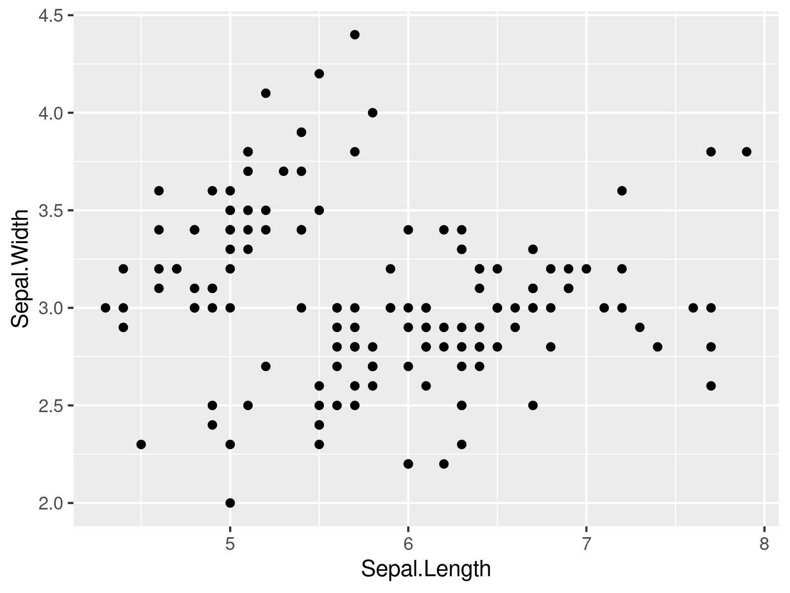
We aim to fit the relationship of Sepal.Length and Sepal.Width.
ggplot(iris, # Plot data aes(x = Sepal.Length, y = Sepal.Width)) + geom_point() |
ggplot(iris, # Plot data aes(x = Sepal.Length, y = Sepal.Width)) + geom_point()

As you can see in the plot, the relationship does not seem to be linear, so lets go for a penalized spline.
We use five equally spaced knots for the spline.
knots <- seq(min(iris$Sepal.Length), max(iris$Sepal.Length), length = 5) # Choose knots |
knots <- seq(min(iris$Sepal.Length), max(iris$Sepal.Length), length = 5) # Choose knots
There are different methods of setting the penalty parameter for a penalized spline. Using package SpatialExtremes, we use the generalized cross validation (GCV) and cross-validation (CV) score. For more information on the scores, we recommend the book the Elements of Statistical Learning by Trevor Hastie, Robert Tibshirani, and Jerome Friedman.
gcv_res <- SpatialExtremes::gcv(y = iris$Sepal.Width, # Calculate GCV x = iris$Sepal.Length, knots = knots, degree = 3) |
gcv_res <- SpatialExtremes::gcv(y = iris$Sepal.Width, # Calculate GCV x = iris$Sepal.Length, knots = knots, degree = 3)
cv_res <- SpatialExtremes::cv(y = iris$Sepal.Width, # Calculate CV x = iris$Sepal.Length, knots = knots, degree = 3) |
cv_res <- SpatialExtremes::cv(y = iris$Sepal.Width, # Calculate CV x = iris$Sepal.Length, knots = knots, degree = 3)
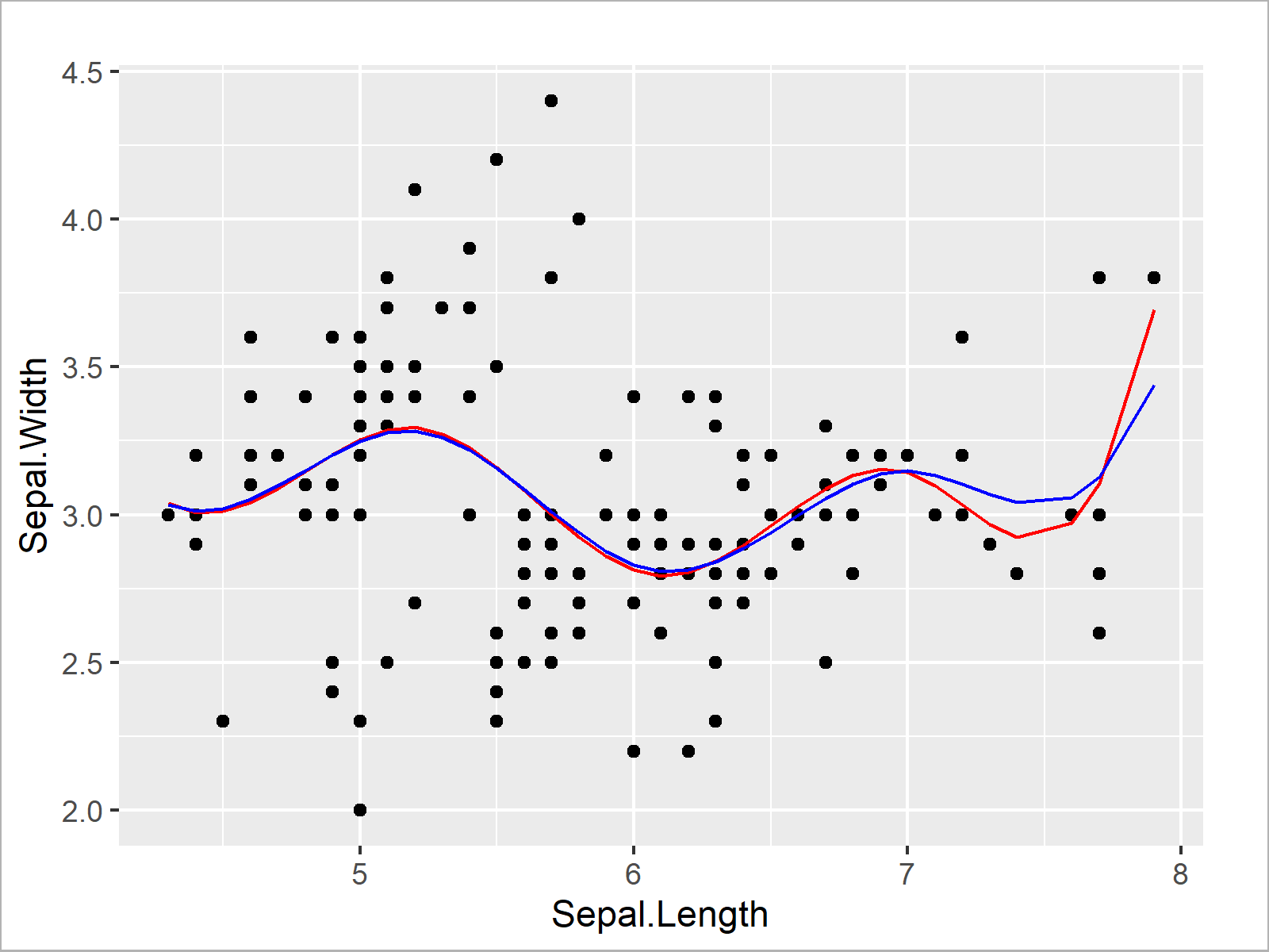
We take a look at the penalty parameter proposed according to the CV and GCV scores.
gcv_res$penalty # Optimal penalty according to GCV # [1] 0.3972609 cv_res$penalty # Optimal penalty according to CV # [1] 0.0007953695 |
gcv_res$penalty # Optimal penalty according to GCV # [1] 0.3972609 cv_res$penalty # Optimal penalty according to CV # [1] 0.0007953695
We visualize the data and the fit of the penalized splines.
cv.fit <- rbpspline(y = iris$Sepal.Width, # CV fit x = iris$Sepal.Length, knots = knots, degree = 3, penalty = "cv") gcv.fit <- rbpspline(y = iris$Sepal.Width, # GCV fit x = iris$Sepal.Length, knots = knots, degree = 3, penalty = "gcv") ggplot(iris, # Plot data # Plot data aes(x = Sepal.Length, y = Sepal.Width)) + geom_point() + geom_line(aes(x = cv.fit$x, y = cv.fit$y), color = "red") + # Add p-spline with penalty chosen with CV geom_line(aes(x = gcv.fit$x, y = gcv.fit$y), color = "blue") # Add p-spline with penalty chosen with GCV |
cv.fit <- rbpspline(y = iris$Sepal.Width, # CV fit x = iris$Sepal.Length, knots = knots, degree = 3, penalty = "cv") gcv.fit <- rbpspline(y = iris$Sepal.Width, # GCV fit x = iris$Sepal.Length, knots = knots, degree = 3, penalty = "gcv") ggplot(iris, # Plot data # Plot data aes(x = Sepal.Length, y = Sepal.Width)) + geom_point() + geom_line(aes(x = cv.fit$x, y = cv.fit$y), color = "red") + # Add p-spline with penalty chosen with CV geom_line(aes(x = gcv.fit$x, y = gcv.fit$y), color = "blue") # Add p-spline with penalty chosen with GCV

Note: This article was created in collaboration with Anna-Lena Wölwer. Anna-Lena is a researcher and programmer who creates tutorials on statistical methodology as well as on the R programming language. You may find more info about Anna-Lena and her other articles on her profile page.

